Getting Started with Tidymodels

When learning things I always like to use Palmer Penguins! It’s a fun dataset and after doing so many projects with iris data or car data it’s nice to change it up.

library(palmerpenguins)
library(tidymodels)
library(tidyverse)
library(ggplot2)

Exploring Data

This is a data set of observations of penguins, and here is a tibble so we can get an overview of what we know about them.

penguins %>% 
    head()

# A tibble: 6 × 7
  species island    bill_length_mm bill_depth_mm flipper_length_mm body_mass_g
  <fct>   <fct>              <dbl>         <dbl>             <int>       <int>
1 Adelie  Torgersen           39.1          18.7               181        3750
2 Adelie  Torgersen           39.5          17.4               186        3800
3 Adelie  Torgersen           40.3          18                 195        3250
4 Adelie  Torgersen           NA            NA                  NA          NA
5 Adelie  Torgersen           36.7          19.3               193        3450
6 Adelie  Torgersen           39.3          20.6               190        3650
# ℹ 1 more variable: sex <fct>

I want to see what the counts for some things are to get a feel for how many NA’s I have as the tibble above shows that some entries are NA.

penguins %>% 
    count(species)

# A tibble: 3 × 2
  species       n
  <fct>     <int>
1 Adelie      152
2 Chinstrap    68
3 Gentoo      124

penguins %>% 
    count(sex)

# A tibble: 3 × 2
  sex        n
  <fct>  <int>
1 female   165
2 male     168
3 <NA>      11

penguins %>% 
    count(island, species)

# A tibble: 5 × 3
  island    species       n
  <fct>     <fct>     <int>
1 Biscoe    Adelie       44
2 Biscoe    Gentoo      124
3 Dream     Adelie       56
4 Dream     Chinstrap    68
5 Torgersen Adelie       52

Okay so I have ~11 entries with NA. I think for this model I’ll try to make a classification model to see if I can corrently predict the sex based on it’s characteristics. I am going to do a little more exploration to see how feasible this is.

penguins %>% 
    filter(!is.na(sex)) %>% 
    ggplot(aes(flipper_length_mm, bill_length_mm, color = sex, size = body_mass_g)) +
    geom_point(alpha = .7) +
    facet_wrap(~species)

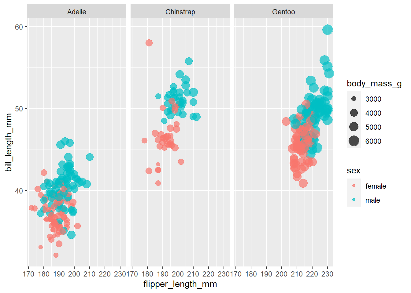
So notice that for all 3 species of penguins, female penguins have smaller bill lengths, flipper lengths and generally less body mass. There is some overlap, but it’s nothing very messy. This seems like some good indication that for all 3 species we can use these two feature to build our classifier. Also interesting that the smallest Gentoo is about as large as the biggest Adelie.

Building A Model

Let’s grab our data and store it in a data frame so we can start to build a model.

penguins_df <- penguins %>% 
    filter(!is.na(sex)) %>% 
    select(-island)

Now to split the data into testing and training sets.

set.seed(777)
penguin_split <- initial_split(penguins_df, strata = sex)
penguin_training <- training(penguin_split)
penguin_testing <- testing(penguin_split)

The default for initial split is a 75% split, and while this isn’t a large data set we can create a resampled data set using the training set to compute the performance of the models that I train. So using boostraps I will create a set of objects each with ~250 training samples and ~90 testing samples (all with resampling) to have a larget dataset to train my classifier with.

set.seed(2134)
penguin_boot <- bootstraps(penguin_training)
penguin_boot

# Bootstrap sampling 
# A tibble: 25 × 2
   splits           id         
   <list>           <chr>      
 1 <split [249/91]> Bootstrap01
 2 <split [249/89]> Bootstrap02
 3 <split [249/89]> Bootstrap03
 4 <split [249/84]> Bootstrap04
 5 <split [249/93]> Bootstrap05
 6 <split [249/82]> Bootstrap06
 7 <split [249/89]> Bootstrap07
 8 <split [249/94]> Bootstrap08
 9 <split [249/92]> Bootstrap09
10 <split [249/96]> Bootstrap10
# ℹ 15 more rows

Now to make a basic logistic regression model and another model. What I am doing with this command is setting up what kind of model I want to train. I haven’t trained it, yet… the other will be a random forest because they usually perform well with their defaults. I am not worried about setting parameters, I just want to try out tinymodels.

library(ranger)
glm_spec <- logistic_reg() %>% 
    set_engine('glm')

rf_spec <- rand_forest() %>% 
    set_mode('classification') %>% 
    set_engine('ranger')

Now it’s time to get this into tinymodels and all working together. I am going to use workflow for this. workflow is a pre-processor and a model.

penguin_wf <- workflow() %>% 
    add_formula(sex ~ .)

penguin_wf

══ Workflow ════════════════════════════════════════════════════════════════════
Preprocessor: Formula
Model: None

── Preprocessor ────────────────────────────────────────────────────────────────
sex ~ .

So notice that when we call this we have a pre=processor, and no model. There is no model yet because I am going to use this to call two times to build both models. I can reuse this workflow as many times as I want for different models which is neat!

glm_results <- penguin_wf %>% 
    add_model(glm_spec) %>% 
    # fit(data = penguins_df) I could do this which would fit the model one time, but I want to use all those resamples I made so I will use fit_resamples instead
    fit_resamples(resamples = penguin_boot,
                                control = control_resamples(save_pred = T, verbose = T)
                                )
glm_results

# Resampling results
# Bootstrap sampling 
# A tibble: 25 × 5
   splits           id          .metrics         .notes           .predictions
   <list>           <chr>       <list>           <list>           <list>      
 1 <split [249/91]> Bootstrap01 <tibble [2 × 4]> <tibble [0 × 3]> <tibble>    
 2 <split [249/89]> Bootstrap02 <tibble [2 × 4]> <tibble [0 × 3]> <tibble>    
 3 <split [249/89]> Bootstrap03 <tibble [2 × 4]> <tibble [0 × 3]> <tibble>    
 4 <split [249/84]> Bootstrap04 <tibble [2 × 4]> <tibble [0 × 3]> <tibble>    
 5 <split [249/93]> Bootstrap05 <tibble [2 × 4]> <tibble [0 × 3]> <tibble>    
 6 <split [249/82]> Bootstrap06 <tibble [2 × 4]> <tibble [0 × 3]> <tibble>    
 7 <split [249/89]> Bootstrap07 <tibble [2 × 4]> <tibble [0 × 3]> <tibble>    
 8 <split [249/94]> Bootstrap08 <tibble [2 × 4]> <tibble [0 × 3]> <tibble>    
 9 <split [249/92]> Bootstrap09 <tibble [2 × 4]> <tibble [1 × 3]> <tibble>    
10 <split [249/96]> Bootstrap10 <tibble [2 × 4]> <tibble [0 × 3]> <tibble>    
# ℹ 15 more rows

There were issues with some computations:

  - Warning(s) x2: glm.fit: fitted probabilities numerically 0 or 1 occurred

Run `show_notes(.Last.tune.result)` for more information.

rf_results <- penguin_wf %>% 
    add_model(rf_spec) %>% 
    fit_resamples(resamples = penguin_boot,
                                control = control_resamples(save_pred = T, verbose = T)
                                )
rf_results

# Resampling results
# Bootstrap sampling 
# A tibble: 25 × 5
   splits           id          .metrics         .notes           .predictions
   <list>           <chr>       <list>           <list>           <list>      
 1 <split [249/91]> Bootstrap01 <tibble [2 × 4]> <tibble [0 × 3]> <tibble>    
 2 <split [249/89]> Bootstrap02 <tibble [2 × 4]> <tibble [0 × 3]> <tibble>    
 3 <split [249/89]> Bootstrap03 <tibble [2 × 4]> <tibble [0 × 3]> <tibble>    
 4 <split [249/84]> Bootstrap04 <tibble [2 × 4]> <tibble [0 × 3]> <tibble>    
 5 <split [249/93]> Bootstrap05 <tibble [2 × 4]> <tibble [0 × 3]> <tibble>    
 6 <split [249/82]> Bootstrap06 <tibble [2 × 4]> <tibble [0 × 3]> <tibble>    
 7 <split [249/89]> Bootstrap07 <tibble [2 × 4]> <tibble [0 × 3]> <tibble>    
 8 <split [249/94]> Bootstrap08 <tibble [2 × 4]> <tibble [0 × 3]> <tibble>    
 9 <split [249/92]> Bootstrap09 <tibble [2 × 4]> <tibble [0 × 3]> <tibble>    
10 <split [249/96]> Bootstrap10 <tibble [2 × 4]> <tibble [0 × 3]> <tibble>    
# ℹ 15 more rows

Now to compare how they did.

collect_metrics(rf_results)

# A tibble: 2 × 6
  .metric  .estimator  mean     n std_err .config             
  <chr>    <chr>      <dbl> <int>   <dbl> <chr>               
1 accuracy binary     0.901    25 0.00426 Preprocessor1_Model1
2 roc_auc  binary     0.964    25 0.00300 Preprocessor1_Model1

# vs
collect_metrics(glm_results)

# A tibble: 2 × 6
  .metric  .estimator  mean     n std_err .config             
  <chr>    <chr>      <dbl> <int>   <dbl> <chr>               
1 accuracy binary     0.910    25 0.00522 Preprocessor1_Model1
2 roc_auc  binary     0.975    25 0.00239 Preprocessor1_Model1

These are very close together, perhaps the same. In this case I’d pick the linear model as it’s easier to interpret and faster to deploy. Since I saved the predictions we can start to look at them in more depth for the linear model.

glm_results %>% 
    conf_mat_resampled()

# A tibble: 4 × 3
  Prediction Truth   Freq
  <fct>      <fct>  <dbl>
1 female     female 40.7 
2 female     male    4.2 
3 male       female  4.08
4 male       male   42.2 

glm_results %>% 
    collect_predictions() %>% 
    group_by(id) %>% 
    roc_curve(sex, .pred_female) %>% 
    ggplot(aes(1 - specificity, sensitivity, color = id)) +
    geom_abline(lty = 2, color = 'gray80', size = 1.5) +
    geom_path(show.legend = F, alpha = 0.9) +
    coord_equal()

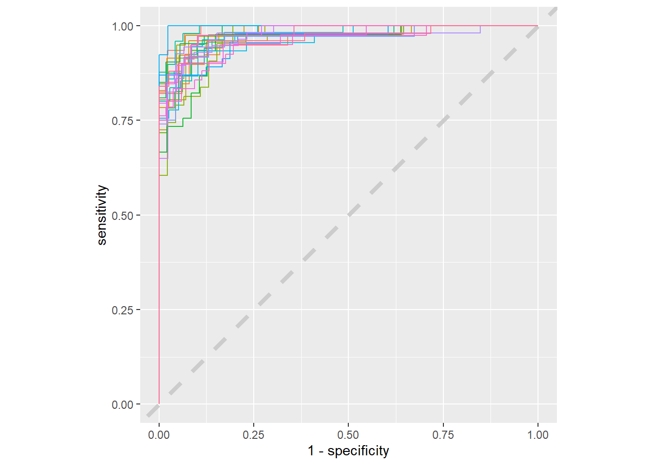
Having more data would make this less jagged, but this gives us an understanding of what the variation is from resample to resample. Things look pretty good, everything is fairly clustered. It passes the smell test. Now it’s finally time to come back to the testing data to estimate the performance on new data. I’ll use the last_fit function to fit the last and best fit to the testing data.

penguin_final <- penguin_wf %>% 
    add_model(glm_spec) %>% 
    last_fit(penguin_split)

collect_metrics(penguin_final)

# A tibble: 2 × 4
  .metric  .estimator .estimate .config             
  <chr>    <chr>          <dbl> <chr>               
1 accuracy binary         0.893 Preprocessor1_Model1
2 roc_auc  binary         0.967 Preprocessor1_Model1

collect_predictions(penguin_final) %>% 
    conf_mat(sex, .pred_class)

          Truth
Prediction female male
    female     40    7
    male        2   35

Not to bad, I can see why some of the females would be classified as males as I did note the overlap in the exploration section. Overall this took less than an hour using packages I’ve never used and having to read the documentation for the workflow of these packages.

I want to take a look at a fitted workflow to see what appears in there now compared to when I last looked at a workflow, and we can look at the odds ratios to see how to interpret this model.

penguin_final$.workflow[[1]]

══ Workflow [trained] ══════════════════════════════════════════════════════════
Preprocessor: Formula
Model: logistic_reg()

── Preprocessor ────────────────────────────────────────────────────────────────
sex ~ .

── Model ───────────────────────────────────────────────────────────────────────

Call:  stats::glm(formula = ..y ~ ., family = stats::binomial, data = data)

Coefficients:
      (Intercept)   speciesChinstrap      speciesGentoo     bill_length_mm  
       -91.797559          -8.434696         -11.983135           0.616936  
    bill_depth_mm  flipper_length_mm        body_mass_g  
         1.462226           0.085003           0.006811  

Degrees of Freedom: 248 Total (i.e. Null);  242 Residual
Null Deviance:      345.2 
Residual Deviance: 90.2     AIC: 104.2

penguin_final$.workflow[[1]] %>% 
    tidy(exponentiate = T) %>% 
    arrange(estimate)

# A tibble: 7 × 5
  term              estimate std.error statistic       p.value
  <chr>                <dbl>     <dbl>     <dbl>         <dbl>
1 (Intercept)       1.36e-40  16.0         -5.75 0.00000000900
2 speciesGentoo     6.25e- 6   3.27        -3.66 0.000253     
3 speciesChinstrap  2.17e- 4   2.05        -4.12 0.0000373    
4 body_mass_g       1.01e+ 0   0.00139      4.89 0.00000101   
5 flipper_length_mm 1.09e+ 0   0.0546       1.56 0.120        
6 bill_length_mm    1.85e+ 0   0.153        4.02 0.0000578    
7 bill_depth_mm     4.32e+ 0   0.375        3.90 0.0000948    

So for every 1 mm increase in bill depth for a penguin the odds of it being a male goes up over 4 times. So the bill depth is very important for penguins being male. I didn’t know that just bill depth would be such a good predictor. Let’s look at those plots from earlier now that we have the odds ratios.

penguins %>% 
    filter(!is.na(sex)) %>% 
    ggplot(aes(flipper_length_mm, bill_length_mm, color = sex, size = body_mass_g)) +
    geom_point(alpha = .7) +
    facet_wrap(~species)

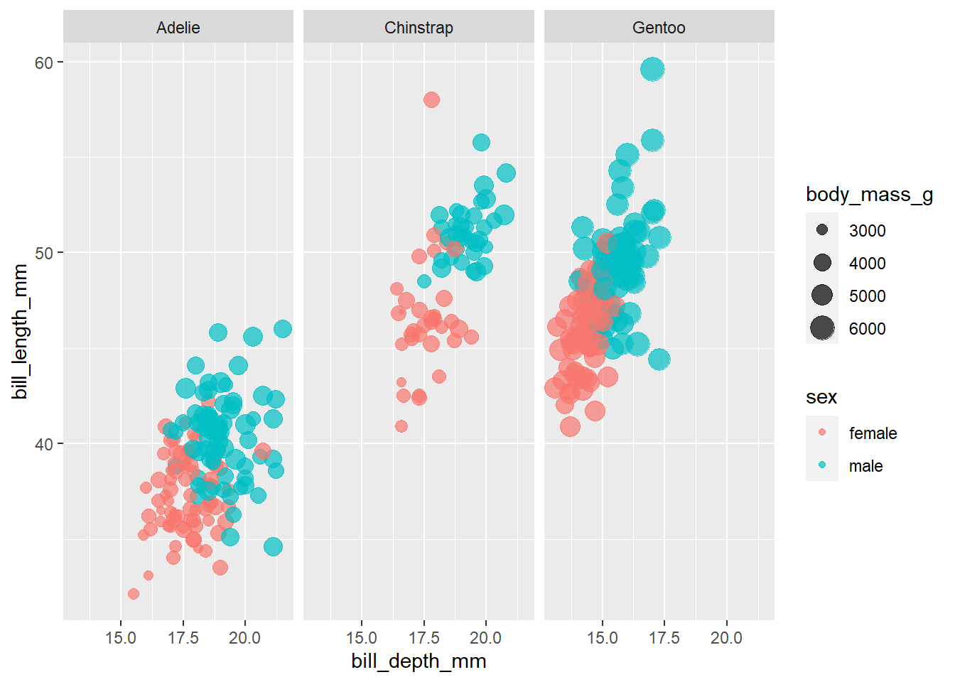
These are pretty overllaped, so now that we know the odds are much better for bill_depth_mm let’s put that on the x-axis and see if the data becomes less clustered.

penguins %>% 
    filter(!is.na(sex)) %>% 
    ggplot(aes(bill_depth_mm, bill_length_mm, color = sex, size = body_mass_g)) +
    geom_point(alpha = .7) +
    facet_wrap(~species)

This does seem to seperate them out more dramatically than flipper_length_mm. Very cool.